#steps 1-6

Load the R packages we will use.

library(tidyverse)
library(echarts4r)  #install this package before using
library(hrbrthemes) #install this package before using

2.Read the data in the files, drug_cos.csv, health_cos.csv in to R and assign to the variables drug_cos and health_cos, respectively

drug_cos <- read_csv("https://estanny.com/static/week6/drug_cos.csv")

health_cos <- read_csv("https://estanny.com/static/week6/health_cos.csv")

Use glimpse to get a glimpse of the data

drug_cos %>% glimpse()

Rows: 104
Columns: 9
$ ticker       <chr> "ZTS", "ZTS", "ZTS", "ZTS", "ZTS", "ZTS", "Z...
$ name         <chr> "Zoetis Inc", "Zoetis Inc", "Zoetis Inc", "Z...
$ location     <chr> "New Jersey; U.S.A", "New Jersey; U.S.A", "N...
$ ebitdamargin <dbl> 0.149, 0.217, 0.222, 0.238, 0.182, 0.335, 0....
$ grossmargin  <dbl> 0.610, 0.640, 0.634, 0.641, 0.635, 0.659, 0....
$ netmargin    <dbl> 0.058, 0.101, 0.111, 0.122, 0.071, 0.168, 0....
$ ros          <dbl> 0.101, 0.171, 0.176, 0.195, 0.140, 0.286, 0....
$ roe          <dbl> 0.069, 0.113, 0.612, 0.465, 0.285, 0.587, 0....
$ year         <dbl> 2011, 2012, 2013, 2014, 2015, 2016, 2017, 20...

health_cos %>% glimpse()

Rows: 464
Columns: 11
$ ticker      <chr> "ZTS", "ZTS", "ZTS", "ZTS", "ZTS", "ZTS", "ZT...
$ name        <chr> "Zoetis Inc", "Zoetis Inc", "Zoetis Inc", "Zo...
$ revenue     <dbl> 4233000000, 4336000000, 4561000000, 478500000...
$ gp          <dbl> 2581000000, 2773000000, 2892000000, 306800000...
$ rnd         <dbl> 427000000, 409000000, 399000000, 396000000, 3...
$ netincome   <dbl> 245000000, 436000000, 504000000, 583000000, 3...
$ assets      <dbl> 5711000000, 6262000000, 6558000000, 658800000...
$ liabilities <dbl> 1975000000, 2221000000, 5596000000, 525100000...
$ marketcap   <dbl> NA, NA, 16345223371, 21572007994, 23860348635...
$ year        <dbl> 2011, 2012, 2013, 2014, 2015, 2016, 2017, 201...
$ industry    <chr> "Drug Manufacturers - Specialty & Generic", "...

4.Which variables are the same in both data sets

names_drug <- drug_cos %>% names()
names_health <- health_cos %>% names()
intersect(names_drug, names_health)

[1] "ticker" "name"   "year"

Select subset of variables to work with

For drug_cos select (in this order): ticker, year, grossmargin

Extract observations for 2018

Assign output to drug_subset

For health_cos select (in this order): ticker, year, revenue, gp, industry

Extract observations for 2018

Assign output to health_subset

drug_subset  <- drug_cos  %>% 
  select(ticker, year, grossmargin)  %>% 
  filter(year == 2018)

health_subset  <- health_cos  %>%
  select(ticker, year, revenue, gp, industry)  %>% 
  filter(year == 2018)

Keep all the rows and columns drug_subset join with columns in health_subset

drug_subset  %>% left_join(health_subset)

# A tibble: 13 x 6
   ticker  year grossmargin   revenue        gp industry              
   <chr>  <dbl>       <dbl>     <dbl>     <dbl> <chr>                 
 1 ZTS     2018       0.672   5.82e 9   3.91e 9 Drug Manufacturers - ~
 2 PRGO    2018       0.387   4.73e 9   1.83e 9 Drug Manufacturers - ~
 3 PFE     2018       0.79    5.36e10   4.24e10 Drug Manufacturers - ~
 4 MYL     2018       0.35    1.14e10   4.00e 9 Drug Manufacturers - ~
 5 MRK     2018       0.681   4.23e10   2.88e10 Drug Manufacturers - ~
 6 LLY     2018       0.738   2.46e10   1.81e10 Drug Manufacturers - ~
 7 JNJ     2018       0.668   8.16e10   5.45e10 Drug Manufacturers - ~
 8 GILD    2018       0.781   2.21e10   1.73e10 Drug Manufacturers - ~
 9 BMY     2018       0.71    2.26e10   1.60e10 Drug Manufacturers - ~
10 BIIB    2018       0.865   1.35e10   1.16e10 Drug Manufacturers - ~
11 AMGN    2018       0.827   2.37e10   1.96e10 Drug Manufacturers - ~
12 AGN     2018       0.861   1.58e10   1.36e10 Drug Manufacturers - ~
13 ABBV    2018       0.764   3.28e10   2.50e10 Drug Manufacturers - ~

Question: join_ticker

Start with drug_cos

Extract observations for the ticker ** MRK** from drug_cos

Assign output to the variable drug_cos_subset

drug_cos_subset  <- drug_cos %>% 
  filter(ticker == "MRK")

Display drug_cos_subset

drug_cos_subset

# A tibble: 8 x 9
  ticker name  location ebitdamargin grossmargin netmargin   ros   roe
  <chr>  <chr> <chr>           <dbl>       <dbl>     <dbl> <dbl> <dbl>
1 MRK    Merc~ New Jer~        0.305       0.649     0.131 0.15  0.114
2 MRK    Merc~ New Jer~        0.33        0.652     0.13  0.182 0.113
3 MRK    Merc~ New Jer~        0.282       0.615     0.1   0.123 0.089
4 MRK    Merc~ New Jer~        0.567       0.603     0.282 0.409 0.248
5 MRK    Merc~ New Jer~        0.298       0.622     0.112 0.136 0.096
6 MRK    Merc~ New Jer~        0.254       0.648     0.098 0.117 0.092
7 MRK    Merc~ New Jer~        0.278       0.678     0.06  0.162 0.063
8 MRK    Merc~ New Jer~        0.313       0.681     0.147 0.206 0.199
# ... with 1 more variable: year <dbl>

Use left_join to combine the rows and columns of drug_cos_subset with the columns of health_cos

Assign the output to combo_df

combo_df  <- drug_cos_subset  %>% 
  left_join(health_cos)

Display combo_df

combo_df

# A tibble: 8 x 17
  ticker name  location ebitdamargin grossmargin netmargin   ros   roe
  <chr>  <chr> <chr>           <dbl>       <dbl>     <dbl> <dbl> <dbl>
1 MRK    Merc~ New Jer~        0.305       0.649     0.131 0.15  0.114
2 MRK    Merc~ New Jer~        0.33        0.652     0.13  0.182 0.113
3 MRK    Merc~ New Jer~        0.282       0.615     0.1   0.123 0.089
4 MRK    Merc~ New Jer~        0.567       0.603     0.282 0.409 0.248
5 MRK    Merc~ New Jer~        0.298       0.622     0.112 0.136 0.096
6 MRK    Merc~ New Jer~        0.254       0.648     0.098 0.117 0.092
7 MRK    Merc~ New Jer~        0.278       0.678     0.06  0.162 0.063
8 MRK    Merc~ New Jer~        0.313       0.681     0.147 0.206 0.199
# ... with 9 more variables: year <dbl>, revenue <dbl>, gp <dbl>,
#   rnd <dbl>, netincome <dbl>, assets <dbl>, liabilities <dbl>,
#   marketcap <dbl>, industry <chr>

Note: the variables ticker, name, location and industry are the same for all the observations

Assign the company name to co_name

co_name <- combo_df  %>% 
  distinct(name) %>% 
  pull()

Assign the company location to co_location

co_location  <- combo_df %>% 
  distinct(location)  %>% 
  pull()

Assign the industry to co_industry group

co_industry  <-combo_df  %>% 
  distinct(industry)  %>% 
  pull()

Put the r inline commands used in the blanks below. When you knit the document the results of the commands will be displayed in your text.

The company Merck & Co Inc is located in New Jersey; U.S.A and is a member of the Drug Manufacturers - General industry group

Start with "combo_df"

elect variables (in this order): year, grossmargin, netmargin, revenue, gp, netincome

Assign the output to combo_df_subset

combo_df_subset  <- combo_df  %>% 
  select(year,grossmargin ,netmargin , 
  revenue, gp, netincome)

Display combo_df_subset

combo_df_subset

# A tibble: 8 x 6
   year grossmargin netmargin     revenue          gp   netincome
  <dbl>       <dbl>     <dbl>       <dbl>       <dbl>       <dbl>
1  2011       0.649     0.131 48047000000 31176000000  6272000000
2  2012       0.652     0.13  47267000000 30821000000  6168000000
3  2013       0.615     0.1   44033000000 27079000000  4404000000
4  2014       0.603     0.282 42237000000 25469000000 11920000000
5  2015       0.622     0.112 39498000000 24564000000  4442000000
6  2016       0.648     0.098 39807000000 25777000000  3920000000
7  2017       0.678     0.06  40122000000 27210000000  2394000000
8  2018       0.681     0.147 42294000000 28785000000  6220000000

Create the variable grossmargin_check to compare with the variable grossmargin. They should be equal.

grossmargin_check = gp / revenue

Create the variable close_enough to check that the absolute value of the difference between grossmargin_check and grossmargin is less than 0.001

combo_df_subset  %>% 
  mutate(grossmargin_check = gp / revenue,
  close_enough = abs(grossmargin_check - grossmargin) < 0.001)

# A tibble: 8 x 8
   year grossmargin netmargin revenue      gp netincome
  <dbl>       <dbl>     <dbl>   <dbl>   <dbl>     <dbl>
1  2011       0.649     0.131 4.80e10 3.12e10   6.27e 9
2  2012       0.652     0.13  4.73e10 3.08e10   6.17e 9
3  2013       0.615     0.1   4.40e10 2.71e10   4.40e 9
4  2014       0.603     0.282 4.22e10 2.55e10   1.19e10
5  2015       0.622     0.112 3.95e10 2.46e10   4.44e 9
6  2016       0.648     0.098 3.98e10 2.58e10   3.92e 9
7  2017       0.678     0.06  4.01e10 2.72e10   2.39e 9
8  2018       0.681     0.147 4.23e10 2.88e10   6.22e 9
# ... with 2 more variables: grossmargin_check <dbl>,
#   close_enough <lgl>

Create the variable netmargin_check to compare with the variable netmargin. They should be equal.

Create the variable close_enough to check that the absolute value of the difference between netmargin_check and netmargin is less than 0.001

combo_df  %>% 
  mutate(netmargin_check = netincome / revenue,
  close_enough = abs(netmargin_check - netmargin) < 0.001)

# A tibble: 8 x 19
  ticker name  location ebitdamargin grossmargin netmargin   ros   roe
  <chr>  <chr> <chr>           <dbl>       <dbl>     <dbl> <dbl> <dbl>
1 MRK    Merc~ New Jer~        0.305       0.649     0.131 0.15  0.114
2 MRK    Merc~ New Jer~        0.33        0.652     0.13  0.182 0.113
3 MRK    Merc~ New Jer~        0.282       0.615     0.1   0.123 0.089
4 MRK    Merc~ New Jer~        0.567       0.603     0.282 0.409 0.248
5 MRK    Merc~ New Jer~        0.298       0.622     0.112 0.136 0.096
6 MRK    Merc~ New Jer~        0.254       0.648     0.098 0.117 0.092
7 MRK    Merc~ New Jer~        0.278       0.678     0.06  0.162 0.063
8 MRK    Merc~ New Jer~        0.313       0.681     0.147 0.206 0.199
# ... with 11 more variables: year <dbl>, revenue <dbl>, gp <dbl>,
#   rnd <dbl>, netincome <dbl>, assets <dbl>, liabilities <dbl>,
#   marketcap <dbl>, industry <chr>, netmargin_check <dbl>,
#   close_enough <lgl>

Question: summarize_industry

Fill in the blanks

Put the command you use in the Rchunks in the Rmd file for this quiz

Use the health_cos data

For each industry calculate

mean_netmargin_percent = mean(netincome/ revenue) * 100 median_netmargin_percent = median(netincome / revenue) * 100 min_netmargin_percent = min(netincome / revenue) * 100 max_netmargin_percent = max(netincome / revenue) * 100

health_cos  %>% 
  group_by(industry)  %>% 
  summarize(mean_netmargin_percent = mean(netincome / revenue) * 100,
            median_netmargin_percent = median(netincome / revenue) * 100,
            min_netmargin_percent = min(netincome  / revenue) * 100,
            max_netmargin_percent = max(netincome  / revenue) * 100) %>% flextable::flextable()

industry	mean_netmargin_percent	median_netmargin_percent	min_netmargin_percent	max_netmargin_percent
Biotechnology	-4.657436	7.621995	-197.4908687	68.804898
Diagnostics & Research	13.139154	12.332079	0.3990080	26.344477
Drug Manufacturers - General	19.358281	19.537586	-34.8658185	100.853774
Drug Manufacturers - Specialty & Generic	5.879275	9.008114	-75.9913646	24.515021
Healthcare Plans	3.283594	3.374305	-0.3052745	6.020508
Medical Care Facilities	6.101918	6.458909	1.3975983	8.304696
Medical Devices	12.363459	14.284582	-56.1180853	49.362818
Medical Distribution	1.700144	1.033174	-0.1016205	4.513858
Medical Instruments & Supplies	12.313479	13.978242	-47.0569354	48.853685

mean_netmargin_percent for the industry Medical Care Facilities is 6.10% median_netmargin_percent for the industry Medical Care Facilities is 6.46% min_netmargin_percentfor the industry Medical Care Facilities is 1.40% max_netmargin_percentfor the industry Medical Care Facilitiesis 8.30%

Question inline_ticker

Fill in the blanks

Use the health_cos data

Extract observations for the ticker BMY from health_cos and assign to the variable health_cos_subset

health_cos_subset  <- health_cos  %>% 
  filter(ticker == "BMY")

Display health_cos_subset

health_cos_subset

# A tibble: 8 x 11
  ticker name  revenue      gp    rnd netincome  assets liabilities
  <chr>  <chr>   <dbl>   <dbl>  <dbl>     <dbl>   <dbl>       <dbl>
1 BMY    Bris~ 2.12e10 1.56e10 3.84e9    3.71e9 3.30e10 17103000000
2 BMY    Bris~ 1.76e10 1.30e10 3.90e9    1.96e9 3.59e10 22259000000
3 BMY    Bris~ 1.64e10 1.18e10 3.73e9    2.56e9 3.86e10 23356000000
4 BMY    Bris~ 1.59e10 1.19e10 4.53e9    2.00e9 3.37e10 18766000000
5 BMY    Bris~ 1.66e10 1.27e10 5.92e9    1.56e9 3.17e10 17324000000
6 BMY    Bris~ 1.94e10 1.45e10 5.01e9    4.46e9 3.37e10 17360000000
7 BMY    Bris~ 2.08e10 1.47e10 6.48e9    1.01e9 3.36e10 21704000000
8 BMY    Bris~ 2.26e10 1.60e10 6.34e9    4.92e9 3.50e10 20859000000
# ... with 3 more variables: marketcap <dbl>, year <dbl>,
#   industry <chr>

In the console, type ?distinct. Go to the help pane to see what distinct does

In the console, type ?pull. Go to the help pane to see what pull does

health_cos_subset  %>% 
  distinct(name) %>%  
  pull(name)

[1] "Bristol Myers Squibb Co"

Assign the output to co_name

co_name<- health_cos_subset  %>% 
  distinct(name) %>% 
  pull(name)

You can take output from your code and include it in your text.

The name of the company with ticker BMY is Bristol Myers Squibb Co

In following chuck

Assign the company’s industry group to the variable co_industry

co_industry  <- health_cos_subset %>% 
  distinct(industry) %>% 
  pull()

This is outside the R chunk. Put the r inline commands used in the blanks below. When you knit the document the results of the commands will be displayed in your text.

The company Bristol Myers Squibb Co is a member of the Drug Manufacturers - General group.

Steps 7-11

Prepare the data for the plots

start with health_cos THEN

group_by industry THEN

calculate the median research and development expenditure as a percent of revenue by industry

assign the output to df

df <- health_cos  %>% 
  group_by(industry)  %>%
  summarize(med_rnd_rev = median(rnd/revenue))

Use glimpse to glimpse the data for the plots

df  %>% glimpse()

Rows: 9
Columns: 2
$ industry    <chr> "Biotechnology", "Diagnostics & Research", "D...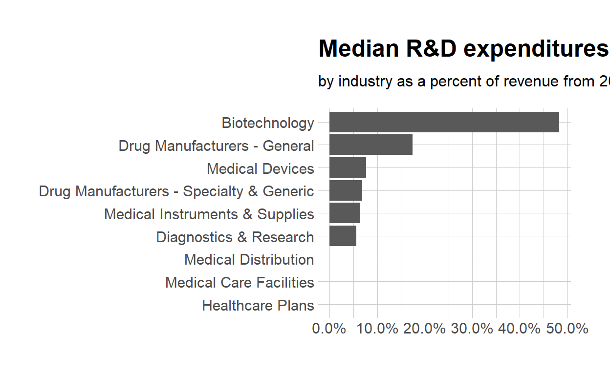
$ med_rnd_rev <dbl> 0.48317287, 0.05620271, 0.17451442, 0.0685187...

Create a static bar chart

use ggplot to initialize the chart

data is df

the variable industry is mapped to the x-axis reorder it based the value of med_rnd_rev

the variable med_rnd_rev is mapped to the y-axis

add a bar chart using geom_col

use scale_y_continuous to label the y-axis with percent

use coord_flip() to flip the coordinates

use labs to add title, subtitle and remove x and y-axes

use theme_ipsum() from the hrbrthemes package to improve the theme

ggplot(data = df, 
       mapping = aes(
         x = reorder(industry, med_rnd_rev ),
         y = med_rnd_rev
         )) +
  geom_col() + 
  scale_y_continuous(labels = scales::percent) +
  coord_flip() +
  labs(
    title = "Median R&D expenditures",
    subtitle = "by industry as a percent of revenue from 2011 to 2018",
    x = NULL, y = NULL) +
  theme_ipsum()

Save the last plot to preview.png and add to the yaml chunk at the top

ggsave(filename = "preview.png", 
       path = here::here("_posts", "2021-03-02-joining-data"))

Create an interactive bar chart using the package [echarts4r] (https://echarts4r.john-coene.com/index.html)

start with the data df

use arrange to reorder med_rnd_rev

use e_charts to initialize a chart the variable industry is mapped to the x-axis

add a bar chart using e_bar with the values of med_rnd_rev

use e_flip_coords() to flip the coordinates

use e_title to add the title and the subtitle

use e_legend to remove the legends

use e_x_axis to change format of labels on x-axis to percent

use e_y_axis to remove labels on y-axis-

use e_theme to change the theme. Find more themes here

df  %>% 
  arrange(med_rnd_rev)  %>%
  e_charts(
    x = industry
    )  %>% 
  e_bar(
    serie = med_rnd_rev, 
    name = "median"
    )  %>%
  e_flip_coords()  %>% 
  e_tooltip()  %>% 
  e_title(
    text = "Median industry R&D expenditures", 
    subtext = "by industry as a percent of revenue from 2011 to 2018",
    left = "center") %>% 
  e_legend(FALSE) %>% 
  e_x_axis(
    formatter = e_axis_formatter("percent", digits = 0)
    )  %>%
  e_y_axis(
    show = FALSE
  )  %>% 
  e_theme("infographic")

Joining data

Question: join_ticker

Question inline_ticker

Steps 7-11